
Definition and function:
One-way analysis of variance is used to study the differences between one categorical variable (X) and one or more quantitative variables (Y). Analysis of variance tests whether different levels of a control variable cause significant differences and changes in the observed variable. For example, whether training has a significant impact on student performance, or whether there are significant differences in performance among candidates from different regions, etc.
Basic assumptions:
In the single-factor experiment, record the factor as A, let there be k levels, denoted as A1, A2, …, Ak, and the variables measured at each level can be regarded as samples from a population. Therefore, there are k populations, the following assumptions need to be satisfied in the analysis of variance:
(1) Each population obeys a normal distribution;
(2) Each population satisfies the homogeneity of variance;
(3) The samples drawn from each population are independent of each other, and there is no multiple linear correlation.
Analysis steps:
(1) Putting forward a hypothesis
Null hypothesis H0: a1 = a2 = … = ak, alternative hypothesis H1: a1, a2, …, ak are not all equal. If the null hypothesis H0 is established, then the influence of different levels of factor A on the indicators is not significantly different; if the null hypothesis H0 is not established, then the influence of different levels of factor A on the indicators is significantly different.
(2) Construct test statistics
First, calculate the mean at different levels of factor A:
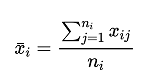
i = 1,2,…k , where ni is the number of the ith overall experimental data;The overall mean of all observations is then determined by taking the mean of all levels:
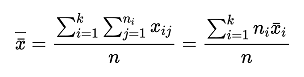
where n = n1 + n2 + … + nk;
The second is to calculate the three error square sum construction test statistics — total error square sum, factor error square sum (intergroup sum of squares) and random error square sum (intragroup sum of squares), respectively SST, SSA, SSE, Its calculation formula is as follows:
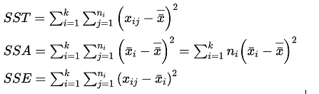
The relationship between these three formulas is SST = SSA + SSE.
In order to ensure the accuracy of the calculation of the error sum of squares, the results of each sum of squares can be divided by the corresponding degrees of freedom to convert them into mean squares for measurement, and the corresponding degrees of freedom are n-1, k-1, and n-k.
The mean square of SSA is also known as the between-group mean square or between-group variance, and is denoted as MSA. The calculation formula can be expressed as MSA = sum of squares between groups/degrees of freedom = SSA / (k – 1);
The mean square of SSE is also known as the within-group mean square or within-group variance, and is denoted as MSE. It is calculated as: MSE = Within Sum of Squares / Degrees of Freedom = SSE/( n – k) .
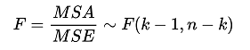
The F test statistic is calculated by dividing MSA by MSE, as shown in the formula below:
(3) Determine the critical value
Given a significance level α, numerator (between-group mean square) degrees of freedom df1 = k – 1, denominator (within-group mean square) degrees of freedom df2 = n – k , find Fα(k – 1,n – k) , to determine the corresponding critical value.
(4) Make a decision
Compare the F value obtained in step (2) with the α level critical value Fα(k – 1, n – k) in step (3), and make a decision. If F > Fα, the null hypothesis is rejected, which means that the hypothesis of H0: a1 = a2 =…= ak is not supported, indicating that the impact of different levels of factor A on the index is significantly different; If F < Fα, the null hypothesis cannot be rejected, and we assume that there is no significant difference in the impact of different levels of factor A on the response variable. When making statistical decisions, you can also directly use the output P value in the variance analysis table to compare with the significance level α to draw a conclusion.
References:
- Kim, T. K. (2017). Understanding one-way ANOVA using conceptual figures. Korean journal of anesthesiology, 70(1), 22-26.
- Quirk, T. J. (2012). One-way analysis of variance (ANOVA). Excel 2007 for Educational and Psychological Statistics: A Guide to Solving Practical Problems, 163-179.
- Heiberger, R. M., & Neuwirth, E. (2009). One-way anova. R through Excel: A spreadsheet interface for statistics, data analysis, and graphics, 165-191.